How to Create Excel Formulas for Random Numbers and Dates
How to use Excel's DATE, RAND and RANDBETWEEN functions to create formulas for random numbers and dates.
Also for sets of random numbers and dates, and for series of dates in date order yet separated by random numbers of days.
Last updated on 2024-05-03.
Preface
For a new spreadsheet, numeric values, dates or both are often needed to test it. Like when a client asked how to populate a set of dates.
In their projects spreadsheet, the client required start and finish dates for each of their projects. For testing, they certainly didn't want to input those dates manually.
In Fill Cells with Random Numbers I've presented a macro for filling cells with random numbers, but what my client required was an Excel formula to do the job.
In this article I'll build up to that particular formula by introducing Excel's RAND, RANDBETWEEN and DATE functions.
Excel's RAND Function
The RAND function has been with Excel since its year dot. Input this formula into a cell and Excel returns a positive decimal number greater than, or equal to, zero and less than one.
=RAND()
That number changes each time you do anything to the spreadsheet to cause it to recalculate.
Excel's RANDBETWEEN Function
Unlike RAND, RANDBETWEEN allows you to specify the upper and lower limits of the range from which you want Excel to return a random number. The function has the two arguments:
RANDBETWEEN(lower_limit, upper_limit)
Input this formula into a cell and Excel returns a positive whole number greater than, or equal to, zero and less than, or equal to 100:
=RANDBETWEEN(0, 100)
This formula with produce numbers between -1000 and 2000:
=RANDBETWEEN(-1000, 2000)
That number changes each time you do anything to the spreadsheet to cause it to recalculate.
Positive and Negative Randomness
Left to itself, RAND generates positive numbers. Putting a minus sign in front of RAND will cause Excel to return negative random numbers, and only negative ones:
=-RAND()
That's why RANDBETWEEN is useful because you can instruct it that you want positive and negative numbers:
=RANDBETWEEN(-1000, 2000)
Excel's DATE Function
Excel works dates based on its built-in calendar which starts in the year 1900 and extends to 9999. If you want to do calculations on dates outside those years, Excel's date functions won't work.
If you input today's date into a cell and then apply the General number format, you'll get a number — probably — that's what Excel calculates to be the number of days since the beginning of 1900.
To calculate the number of days between two dates, your formula takes this form:
=date2-date1
However, for obvious reasons, inputting this formula does not have Excel calculating there are 365 days in 2019:
=(2019-12-31)-(2019-01-01)+1
If you need to introduce a date directly into a formula, you engage the DATE function to cause Excel to refer to its internal calendar. DATE has this structure:
DATE(year, month, day)
It's best to input a four-digit number for year to make certain Excel understands to which century you're referring. (Otherwise, how can you be certain that if, for example, you input 99 as the year, to which century is Excel assigning that year?)
month is a number from one to 12; day a number that is the day of your chosen month.
The order of the arguments is always the same, whatever the regional setting of your computer or the date format you're using. Hence DATE is a useful reassurance that your dates will travel anywhere, uncorrupted.
So, a formula for the number of days in is this:
=DATE(,12,31)-DATE(,1,1)+1
To produce random dates, we'll need to use Excel's DATE function.
A Random Date
Here's a formula for creating a random number that represents a day in Excel's built-in calendar for the year 2019:
=RANDBETWEEN(DATE(2019,1,1),DATE(2019,12,31))
You'll need to ensure that you apply a date format to the cell containing the formula. That number, and therefore your date, will change each time you do anything to the spreadsheet to cause it to recalculate.
Dates for Projects
Now we're set to create a set of dates as required by my client for their projects in 2019 as explained in the Preface:
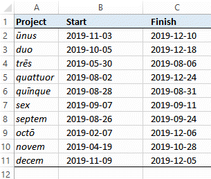
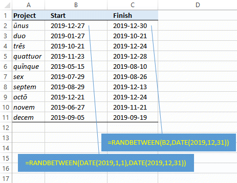
All the dates are randomised. Be that as it may, the random Finish date must be later than the random Start date. Here's my suggestion for the formulas to achieve this:
Duration in Days
My client also needed the duration of each project. That's calculated by subtracting the Start date from the Finish date. Or you might use this as an excuse to engage Excel's DAYS function:
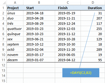
This is the function's structure: DAYS(end_date, start_date).
Revised Project Dates
The Dates for Projects, above, proved unsatisfactory in a couple of respects. These were that each project had to start later than the start of the previous one and that all projects were to start within the current year — make that 2019 in this example.
Leaving the formulas in columns C and D as they were, I set about priming a January start for the first project, inputting this formula in cell B2:
=RANDBETWEEN(DATE(2019,1,1),DATE(2019,1,31)).
Then I seeded the rest of the Start dates by copying down this formula from cell B3:
=RANDBETWEEN(B2,DATE(2019,12,31))
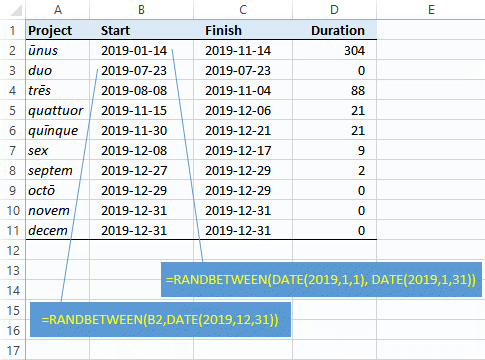
What a disappointment, to say the least! However many times you press key F9 to cause the formulas to recalculate, the dates and durations for those projects later in the list remained out of whack:
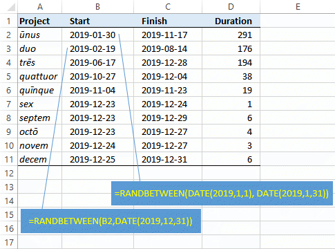
Next to experiment with with this foruula:
=B2+RANDBETWEEN(6,60)
It's OK provided you're patient enough to keep pressing F9 to update the formula results to keep the Start dates within 2019:
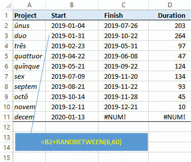
Potential for a repetitive strain injury if you're F9 activity has to get too labourious. So, more work to be done.
A Fresh Approach
Since I first posted on this subject I left it to my subconscious to come up with improved solutions, having set it these objectives:
- As near as can be, 20 pairs of project dates
- Those 20 projects to start in the same year
- Durations to be of similar magnitudes.
This is what came to mind:
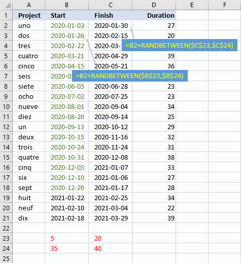
The figures in red af the bottom of the two date columns are the ones you tweak to produce an acceptible data set.
The conditional format on Cells B2 to B21 turns their content green for dates in 2020. This touch makes it easy to spot the the results of your tweaks.
Your Support for DMW TIPS
Please support this website by making a donation to help keep it free of advertising and to help towards cost of time spent adding new content.
To make a contribution by PayPal in GBP (£ sterling) —
To make a contribution by PayPal in USD ($ US) —
