How to Show a Formula Result in a Microsoft® Excel Chart Legend.

Last updated on 2024-05-02.

Question From Client

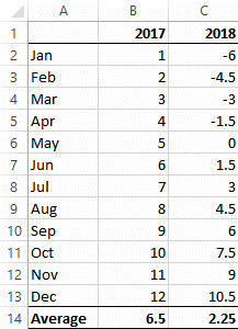
“I have used this table for a chart and want the legend to show ‘2017 - Average 6.50' and ‘2018 - Average 2.25'. The years and the averages in the legend must follow any changes that will occur in the table. Is there a way of doing this?”

Suggestion

Here's one way of making your legend follow the years in row one and the averages in row 14.

First of all, create this formula in a blank cell, e.g. A17:

=TEXT(B1,"0000")&" - Average "&TEXT(B14,"0.00")

Then create this formula in say A18:

=TEXT(C1,"0000")&" - Average "&TEXT(C14,"0.00")

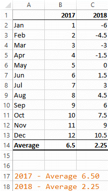
These two formulae generate the legend you want to achieve, making use of the TEXT function to determine the formatting of the numbers involved. Now to make the chart respond to them:

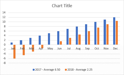
1. Click the chart
2. Click one of the bars in the 2017 figures
3. In the formula bar you will see =SERIES(Sheet4!$B$1,Sheet4!$A$2:$A$13,Sheet4!$B$2:$B$13,1)
4. Make the first argument in the SERIES function reference cell A17, instead of the $B$1
5. Repeat for a 2018 bar, pointing the first argument of its SERIES to cell A18.

Now you should have a legend that looks like this:

Your Support for DMW TIPS

Please support this website by making a donation to help keep it free of advertising and to help towards cost of time spent adding new content.

To make a contribution by PayPal in GBP (£ sterling) —

To make a contribution by PayPal in USD ($ US) —

Thanks, in anticipation.

Disclaimer

David Wallis does not accept any liability for loss or damage to data to which any techniques, methods or code included in this website are applied. Back up your data; test thoroughly before using on live data.